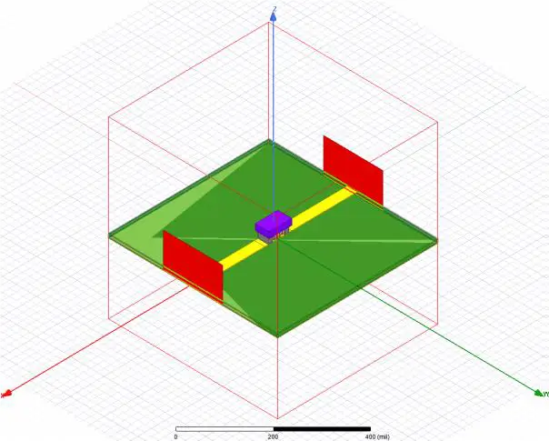
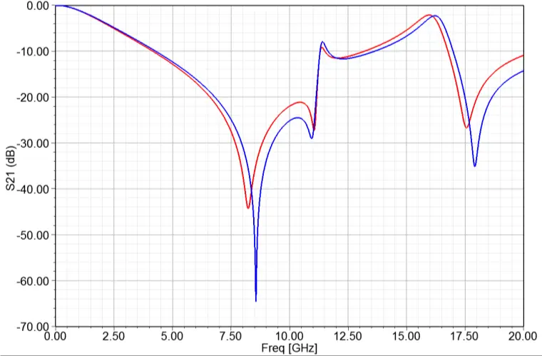
The combination of circuit simulation, equivalent circuit models, and planar electromagnetic (EM) simulation of a PCB layout is typically sufficient for lower frequency designs using surface mount passive components (or discrete or MMIC active devices that are not packed into a compact layout). However, once components are placed in close proximity and design frequencies are increased into the RF/microwave range, this approach no longer captures all of the interactions that will be present in the fabricated design. For these designs, 3D simulation is required for accurate prediction of a circuit’s performance. As powerful of a technique as it is, 3D model and simulation setup is not trivial, requiring a high degree of expertise and in-depth knowledge of the components in the simulation. As such, a pure 3D simulation may not always be practical for all designers. This application note seeks to demonstrate when 3D simulations are required, when planar EM simulations may suffice, and an alternative method to full 3D simulation for capacitors that still manages to capture component coupling effects. Also included in this document is a brief overview of some guidance on 3D simulation setups and overcoming common 3D simulation challenges.
The Need for 3D Simulation
For more compact, complex, or high frequency designs, 3D EM simulation may be needed to best capture circuit performance. In particular, unintended coupling effects between components and their environment can cost designers not using 3D EM simulation large amounts of time and money to fabricate and test multiple versions of a design when the initial attempt fails to meet specification. The most significant sources contributing to coupling effects can be difficult to pinpoint without using 3D EM tools to visualize electric and magnetic fields. Whether component-to-component coupling, component coupling to adjacent lines, or shielding effects are occurring in a given design, 3D EM analysis is a proven method with years of development leading to excellent prediction of measurement results.
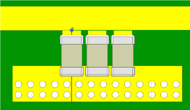
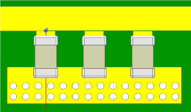
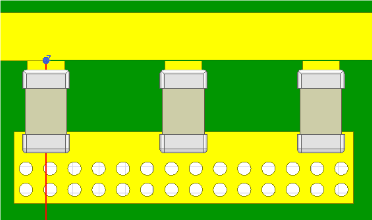
Figure 1 – Three capacitors placed in shunt configuration on a 50 ohm line with the spacing between them varied. Left – Closest spacing between components (10 mils), Center – middle spacing between components (42 mils), Right – furthest spacing between components (74 mils).
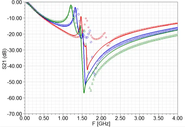
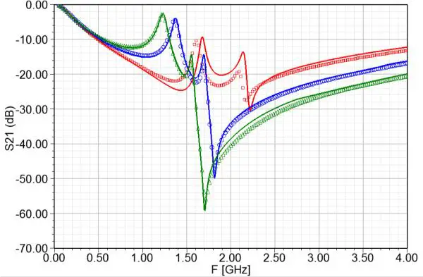
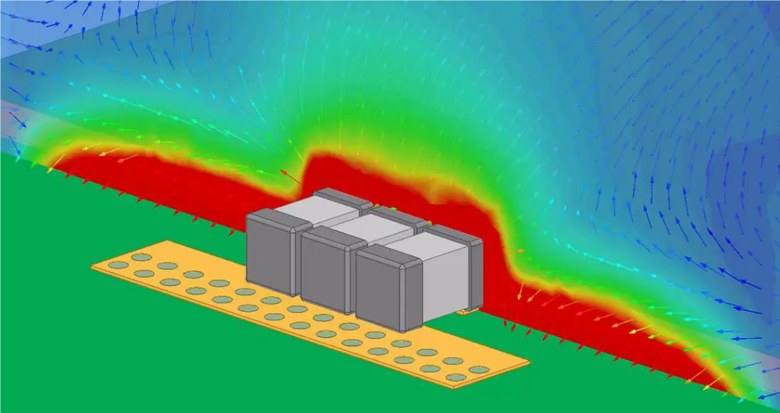
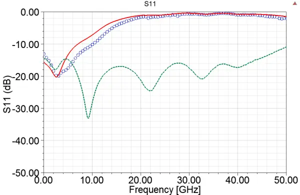
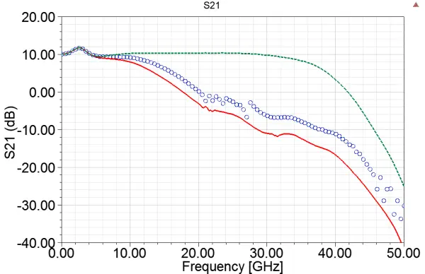
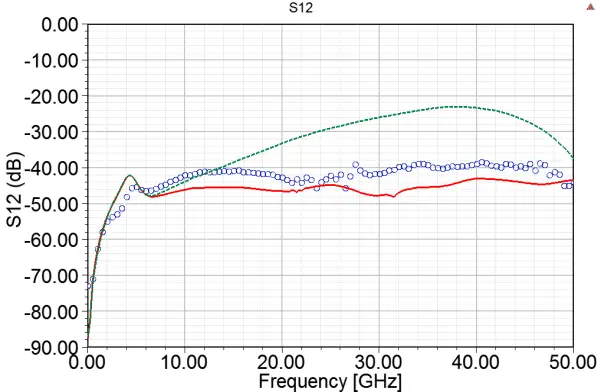
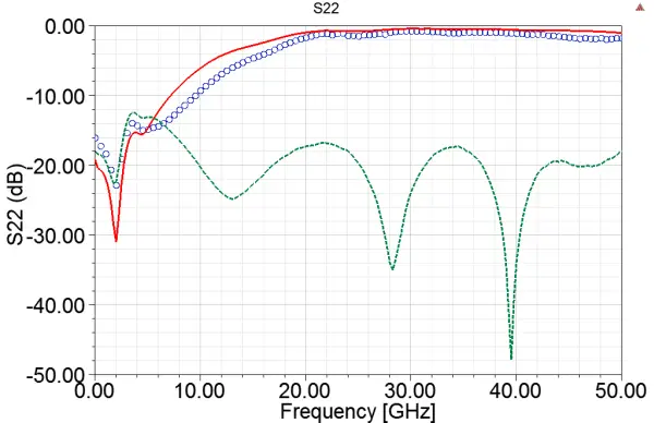
To illustrate this, Figure 1 shows three simple example circuits on a 16mil Rogers 4003C substrate. Surface mount capacitors were placed in shunt configuration on a 50 Ohm line (Capacitor model: 12pF Johanson R14S, Modelithics model number: CAP-JOH-0603-101). The spacing between the components was varied from approximately 1 to 5 substrate heights. A circuit simulation version as well as a 3D version of these circuits was performed in Figure 2 and compared against measured data. The 3D simulation shows excellent agreement with the measured data, accurately tracking the shifting resonances due to proximity effects. The E-field plot shown in Figure 3 clearly demonstrates the component to component coupling taking place in this example.
Figure 2 – Comparison against measured data for capacitor spacings shown in Figure 1. Left – Circuit simulation. Right – 3D EM simulation. Red – Closest spacing between components, blue – middle spacing between components, green – furthest spacing between components.
Figure 3 – Figure 2 Comparison against measured data for capacitor spacings shown in Figure 1. Left – Circuit simulation. Right – 3D EM simulation. Red – Closest spacing between components, blue – middle spacing between components, green – furthest spacing between components. Figure 3 E-field visualization of shunt capacitors with closest spacing shows component-to-component coupling.
Planar EM Co-Simulation and Its Success
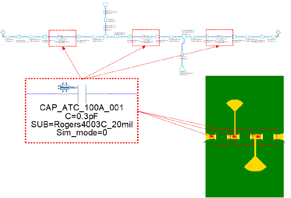
Not all designs require the use of 3D simulation tools for good simulation and measurement correlation. This section presents an example 5GHz elliptic high-pass filter (originally designed using Nuhertz Technology’s FilterSolutions software) where equivalent circuit models and planar EM co-simulation were able to accurately predict the fabricated circuit performance once measured. This particular filter was built on a 20mil Rogers 4003C board and uses a combination of surface mount capacitors and radial stubs to achieve the desired filter response (Figure 4).
Figure 4 – 5GHz elliptic high-pass filter design. Top – circuit simulation representation. Bottom – Layout for filter design used in planar EM co-simulation.
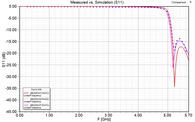
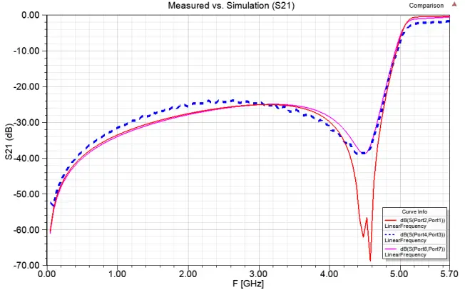
Shown in Figure 5, the measurement data for the 5GHz filter is compared to circuit simulation as well as planar EM co-simulation results. In this case, the lumped and distributed components were separated by enough distance for this application that the equivalent circuit models and planar EM alone gave excellent results.
Figure 5 – Simulation vs measurement comparison for 5GHz elliptic high-pass filter. Dashed blue line – measurement data.Red – circuit simulation results.Magenta – planar EM co-simulation results.
Facilitating these sorts of simulations, Modelithics Microwave Global Models™ are highly scalable equivalent circuit models containing a number of useful simulation features. One such feature being advanced simulation and pad treatment modes which allow for the de-embedding of solder pads, making them easy and accurate for use in EM co-simulations. See Application Note 052 & 054 for more details on the 5GHz elliptic high-pass filter design and how to use Modelithics models in EM co-simulation in HFSS.
An Alternative to Full 3D Simulation: 3D Co-Simulation Using “Brick Models”
Modelithics has developed a path for performing 3D electromagnetic (EM) co-simulation in HFSS using 3D designs and combining these results with Modelithics’ CLR Library models. While the methods for planar EM co-simulation described in other Modelithics application notes can provide good simulation to measurement agreement for most structures, it is not capable of accounting for coupling between the components themselves and between the components and their environment. The method described in this section provides a simple method to capture these coupling effects in simulation.
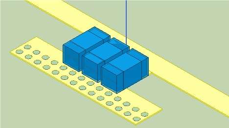
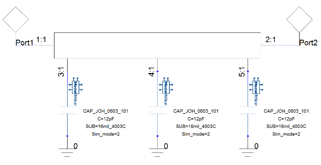
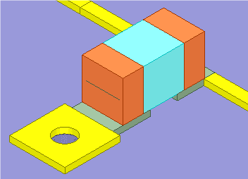
To perform 3D EM co-simulations, an approximation to the physical geometry of the capacitor is setup carefully in the 3D environment. This is what will be referred to as a 3D “brick” model. The full 3D design, including all layout elements, is simulated with the brick model in place of any capacitors. Once the EM simulation is complete, the data is brought into the Nexxim (ANSYS Electronic Desktop’s circuit simulation tool) circuit design and the EM co-simulation is performed by connecting Modelithics’ Microwave Global Models1 to the ports made accessible by the brick model (Figure 6). The Microwave Global Models will now account for the component’s parasitic effects that were left out of the 3D simulation by the brick model.
The beauty of this method is that only a single run of the time-consuming 3D simulation must be performed and the capacitor value can be adjusted after the fact in the circuit simulation. This method provides reasonable results when compared to measured data and allows the user to see coupling effects between capacitors observed in the measured data without needing all of the internal details of the capacitor. This is a significant advantage as it is a fairly arduous task to acquire and properly setup the detailed metalization geometries for multi-layer capacitors. This approach also drastically reduces simulation time as MLCC capacitors’ internal geometry is often complex, typically requiring a fine mesh and long simulation times. It also avoids multiple runs of the 3D simulation when trying different capacitance values. NOTE: This method currently only has been validated for capacitor simulations.
Figure 6 – Left – 0603 sized 3D Brick Models in HFSS 3D Modeler. Right – Co-simulation with CLR models in circuit simulator
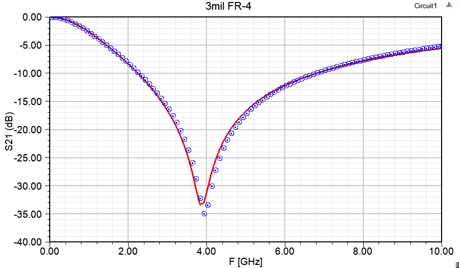
As a proof of concept, the results of using the 3D co-simulation technique for a single capacitor should work just as well as using the technique for multiple coupled capacitors. In this example, an 0201 brick model is simulated on a shunt structure on a 3mil FR-4 substrate. In the circuit simulator, the Microwave Global Model for the 5.6pF Murata GRM033 (CAP-MUR-0201-302) is connected to the 3D SNP data. The 3D co-simulation shows good agreement with the measured data in Figure 7.
Figure 7 – Left – Brick model 3D simulation of single 0201 capacitor mounted in shunt configuration on a 3mil FR-4 substrate. Right – 3D Co-simulation result using the Microwave Global Model for the 5.6pF Murata GRM033 capacitor.
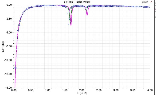
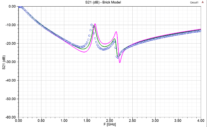
The next example shows a comparison of a full 3D simulation versus the results using the 3D co-simulation method. In Figure 6, 0603 sized brick models were simulated in the same configuration as was done in Figure 1. The Microwave Global Model for the 12pF Johanson R14S (CAP-JOH-0603-101) was then connected in the co-simulation schematic and the result was compared to measured data for the closest spacing between components (10mils). Figure 8 shows that for this case, which would presumably have the strongest component-to-component interaction, the full 3D simulation and the 3D co-simulation both show excellent agreement with the measured data.
Figure 8 – The results comparing simulations of three 12pF capacitors in shunt configuration on 16mil Rogers 4003C using: magenta – full 3D model , green – 3D co-simulation, blue – measured data. Capacitor separation is 10 mils, the closest spacing studied for this configuration.
Common Issues With 3D Simulations
One of the main problems in using 3D EM simulations in a design flow lies in obtaining all of the necessary physical and material properties to enable analysis of the complete circuit. This information is typically proprietary manufacturer intellectual property (IP). Even if all of the physical parameters and material properties are available to the designer, initial 3D model results may not be good when compared to measurement data and tuning of model parameters, mesh, and potentially port setup configuration is often required. Likely sources of model to measurement discrepancies would be uncertainty and fabrication tolerances in the component 3D geometry details, or uncertainty and tolerances in material properties. For this reason, measurement validation of EM models prior to their use for design as well as EM simulation expertise is crucial.
One way to mitigate some of these issues is to use a library of validated and encrypted 3D component models, such as Modelithics’ COMPLETE+3D Library. Modelithics’ 3D models have been encrypted using ANSYS HFSS’s proprietary technology, which allows for the distribution of accurate 3D models to 3rd party customers while maintaining the security of manufacturer IP.
Placing Modelithcs Encrypted 3D Component Models in an HFSS Design
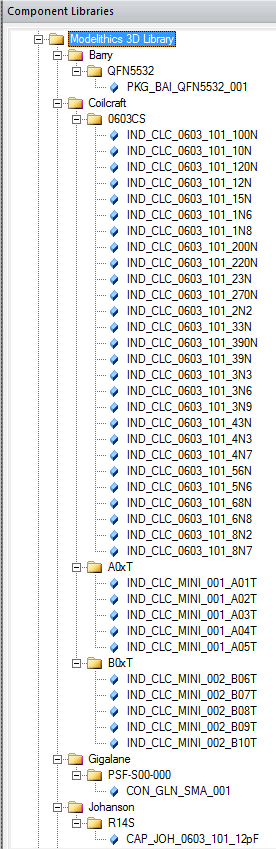
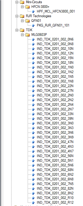
Users taking advantage of the Modelithics COMPLETE+3D Library can quickly and easily begin using measurement-validated 3D models in their designs. Once the library is installed, the encrypted 3D models can be found in the HFSS Component Library window. The available models are organized by manufacturer (Figure 9). To view all of the models, each manufacturer folder can be expanded by clicking the plus (+) sign. A brief model description identifies the manufacturer part number and part value range. In addition all of the Modelithics equivalent circuit models, including Microwave Global Models, available for use in HFSS are included with this installation enabling accurate circuit simulations as well as EM Co-simulations involving the modeled components.
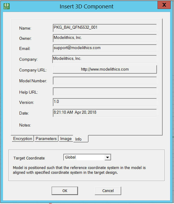
To place a 3D component model, either highlight the desired component and drag and drop into the Modeler window, or right-click on the component and select “Place Component.” A dialog window (Figure 10) will open with information about the 3D model, a model image, and any parameters that are accessible to the user. Clicking “OK” will place the component in the Modeler window depending on the selected coordinate system. The component datasheet can be accesses by either clicking on the link in the component dialog window, or by clicking on the Modelithics logo in the top right corner of the 3D modeler viewing area once the 3D component is added to a design.
Figure 9 – Section of the Modelithics 3D Library in the HFSS Component window.
Figure 10 – The Insert 3D Component window will open when placing a component in the Modeler window.
Port Selection and Setup
Assuming that the 3D component models are accurate, designers still need to integrate their layout into the 3D environment and find the most appropriate way to excite the circuit with ports. There are many port types available in HFSS but generally, either lumped ports or wave ports are the most appropriate to use to excite a PCB-based 3D structure, and both options give similar results (Figure 12). Depending on the layout itself and whether the ability to shift reference planes is needed, different port setups have their own advantages. If the reference planes of the simulation are internal to the model and do not need to be shifted, lumped ports are simple and quick to setup. If the ports are external to the model or if the reference planes need to shift, wave ports may be a more appropriate choice (Figure 11).
Figure 11 – Comparison of port type configuration for 10nH Coilcraft 0603CS inductor (IND-CLC-0603-101) on 10mil Rogers 5880 using lumped ports (left) and wave ports (right).
Figure 12 – 3D simulation of 10nH Coilcraft 0603CS inductor (IND-CLC-0603-101) on 10mil Rogers 5880 using lumped ports (blue trace) and wave ports (red trace).
Guidance on Solution Setups
Older versions of HFSS required the user to do a bit of trial and error to ensure that an appropriate solution frequency was being used to mesh and simulate a design. For example, in a resonant structure, the solution frequency should be set to the design frequency for that structure. The reason to choose the resonant frequency as the solution frequency is that the adaptive meshing process used by HFSS analyzes the mesh for large field differences between adjacent mesh elements. The mesh is refined with each pass until the change in S-Parameters meets the user specified convergence criteria. If the fields or transmission for a structure are very low at the chosen solution frequency, there may not be much difference between adjacent elements and the mesh may converge prematurely. At a resonant frequency, the fields are strongest so the adaptive mesh process is most likely to converge on an accurate mesh for that structure. The user had to be even more careful when dealing with broadband structures or structures where the resonant frequencies are unknown. The user could hypothetically choose any frequency in the band of interest. The highest frequency in the sweep would be a good initial selection, or the approximate frequency of first resonance (if it is known). Regardless, the user would have to investigate the effect of selecting different solution frequencies on the results as well as the maximum number of passes and maximum delta S to converge on an appropriate mesh and ensure a good end result.
But with more recent releases (starting in 2017), multi-frequency adapt meshing technologies were introduced which use multiple frequencies, solved in parallel, for performing the adaptive meshing. For example, a filter designer might elect to perform frequency adaption at the poles of their filter’s designs. The other method introduced is broadband adaptive meshing, which further simplifies the user’s responsibilities in solution frequency selection. All the user must do is specify the frequency sweep of interest and then HFSS will automatically use its own experience in select meshing frequencies for a given sweep definition and even running and extracting multiple in parallel if enough resources are made available to the solution process.
Finally in 2019R2, HFSS extended the broadband adaptive meshing concept to a new auto solution setup mode where the user only needs to specify the sweep definition and then simply use the provided slider bar setting to select the balance between speed and fidelity of simulation is desired. HFSS’s advances in solution setup create a very easy work flow for the user, not requiring them to agonize over the frequencies at which to mesh or the numerical settings necessary for convergence.
Imported Geometry Issues
If the designer is bringing a layout or a specific component model into the HFSS 3D environment from another tool, there can be initial difficulties in integrating these elements due to geometry issues. For example, a common error encountered with imported CAD files is non-manifold geometry errors that manifest once meshing is attempted. Other examples of commonly encountered errors would be non-manifold vertices and edges. The “Heal” function in HFSS may be able to resolve some of these issues, but re-drawing the geometry within HFSS may still be required depending on the severity of the defect.
Tolerances in model geometry and material properties
Manufacturing tolerances on physical dimensions or material properties can cause discrepancies in simulation results, especially when comparing against measurement data. If a fabricated version of the structure is available, a detailed inspection of the actual line/pad/feature dimensions can be useful to help track down possible causes for the differences between simulation and measurement. Unfortunately, material property variation can be harder to isolate and practically impossible to identify by physical inspection. In such a case, the 3D model can be used to study the effect of material property variation. Tolerances can be added to the 3D model and then a parametric analysis (or analytical derivatives) can be used to study changes in performance with respect to dielectric constant or loss tangent, for example.
Application Example
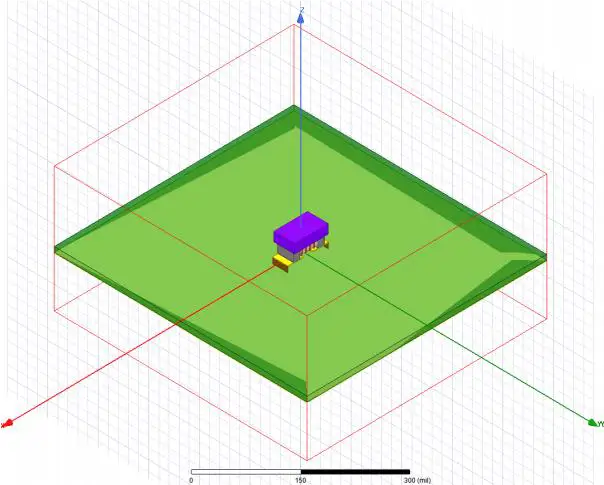
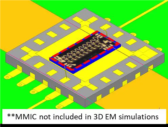
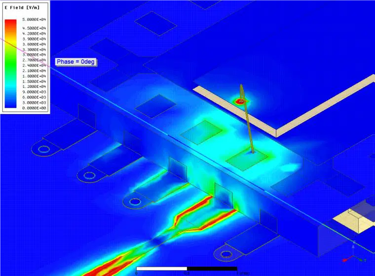
A simulation making best use of computational resources takes advantage of the different strengths of circuit simulation using S-Parameters, equivalent circuit models, and EM analysis. In that respect, 3D EM analysis is not a complete replacement for other simulation methods and tools. 3D EM analysis comes at the cost of an increase in simulation time and is best used in the final stages of the design process to verify that EM interactions will not cause a failure when fabrication is complete. A good example of this can be seen in Figure 13, Figure 14, and Figure 15 where a MMIC amplifier was mounted in an RJR 4mm QFN package. 3D co-simulation of the structure was performed using both S-Parameter data and 3D EM simulation data with good agreement with measurement data.
Figure 13 – Visualization of 3D co-simulation of MMIC amplifier in RJR 4mm QFN package. Package, bondwires and alumina motherboard were simulated in HFSS with ports added to enable co-simulation. Measured S-Parameters of MMIC amplifier were connected to ports in EM simulation.
Figure 14 – E-field visualization of package and bondwire mounted on alumina motherboard shows some coupling between the bondwire and adjacent package pin.
Conclusion
3D EM analysis of structures is an extremely powerful tool in the hands of the experienced designer. Full wave simulators like Ansys HFSS offer designers the unique ability to rigorously test their circuits prior to fabrication for electromagnetic coupling and interaction between components, giving them best chance possible at first pass design success. As powerful as this method is, this is not to say that 3D EM analysis is a complete replacement for other simulation methods and tools. 3D EM analysis comes with a significant time cost to the designer in both setup and simulation, and should be used in the final stages of the design process to verify that EM interactions will not cause failure to meet specification. With the advances in every release of HFSS and using highly accurate models from Modelithics, even newcomers to EM analysis can obtain excellent results and gain meaningful insight into their designs.
About this note:
This application note was developed by Isabella Bedford, Eric Valentino, and Dr. Larry Dunleavy of Modelithics. The authors would like to thank Chris DeMartino of Modelithics and Dr. Matt Commens of Ansys for their helpful editing comments. of Modelithics, Inc. The authors would like to thank Chris DeMartino of Modelithics and Dr. Matt Commens of Ansys for their helpful editing comments.
Contact Information:
For information about Modelithics’ products and services, please contact us at:
Address: Modelithics, Inc. 3802 Spectrum Blvd., Suite 130 Tampa, FL 33612 Voice: 888-359-6539 Email: sales@modelithics.com Web: www.modelithics.com