This application note presents a method for improved design flow with a goal of cost-effective first-pass design success. Typically, when an RF/Microwave design has to be fine-tuned to fit the design criteria, a design engineer will use the built-in optimization capability in the EDA tool. In a typical case, the optimization engine has to deal with ten or more variables such as component values that can be changed, and at least three to four goals. In the case of a microwave filter, example goals would include in-band insertion loss and return loss, cutoff frequency and out of band rejection. The large number of criteria that the optimization engine has to deal with creates a landscape of ” solutions ” that are more or less random. No matter which optimization engine one will use, not all possible outcomes will be tested simply because this would be too time consuming.
In this paper we propose a solution that maps the impact that individual components have on sub-system performance so that a good trade-off can be made with regard to component values and tolerance (low tolerance=more expensive, larger tolerance=less expensive). This will ultimately lead to lower manufacturing costs and improved yield. The proposed solution requires accurate passive component models that allow yield analysis by means of a tolerance setting, something that is close to impossible with commonly used S-Parameter file-based component representations. By combining Modelithics Global Models™ for passive RLC components [1] with AWR microwave Office we allow the software to find an optimal solution that does not only reach the design goal, but will also help the design engineer find an optimum component trade-off and a high yield.
Modelithics CLR Library
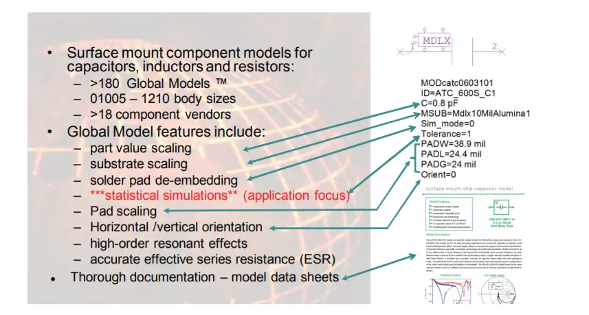
The Modelithics CLR Library offers a wide range of highly scalable Global Models™, each representing an entire family of component values that are scalable based on part-value, substrate and pad dimension properties. The models are also structured to allow for statistical tolerance analysis. All models are thoroughly documented with a detailed model data sheet. Figure 1 summarizes the features of the CLR library and gives an example of a Modelithics capacitor model.
Figure 1: Overview of the features of Modelithics CLR Library “Global Models”.
Low Pass Filter (LPF) Design Goals
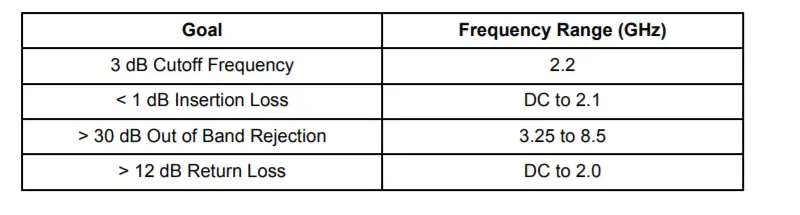
A standard low-pass filter design will be used to demonstrate the proposed new design flow approach, which involves a simulation-based methodology for yield estimation and cost-effective yield improvement. Table 1 shows the design goals for this LPF example. The combination of Modelithics Global models and AWR Design Environment statistical tools provides a clear advantage over the use of commonly available S-Parameter models and traditional design flows.
Table 1: LPF Design Goals
Filter Design Flow
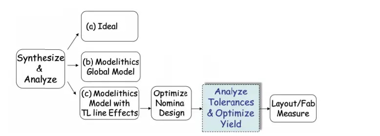
Figure 2 illustrates the proposed filter design flow. It begins with synthesis of an ideal filter. The next step is to step is to substitute the ideal components with Global Models and eventually add transmission line effects. An optimization of part values is then done to compensate for non-idealities and parasitic effects. The result at this point should be a nominal filter design that has a good match to the goals. Transmission line dimensions can be also optimized along with the part-values to fine tune the design and compensate for the lack of availability of in-between part-values that may be required for a more optimal design.
An improvement to this flow, which is the focus of this application note, is to add a tolerance analysis and yield optimization step prior to fabrication. An EM analysis can also be added to further validate the nominal design simulations, however, built-in transmission line models may be more convenient and computationally efficient to use for tolerance analysis.
The design was synthesized by selecting a 5th order Cherbychev filter, with a pass-band ripple of 0.5 dB and a series inductor as a first component. Such designs can be synthesized using filter design tables documented in standard texts [2] or using filter synthesis software routines that are now available in modern microwave electronic design automation tools, such as AWR’s “i-Filter Wizard [3]”.
Figure 2: Suggested Filter Design Flow
LPF Measurement to Model Comparison
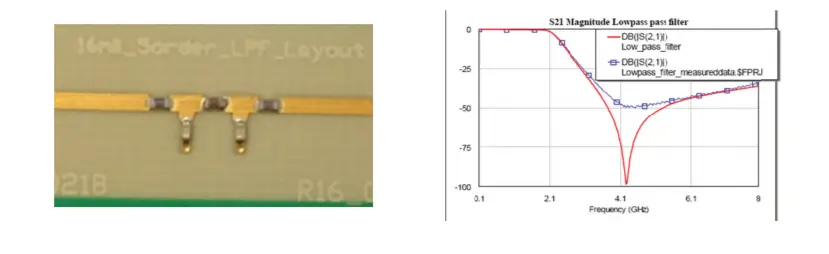
Figure 3 shows the fabricated test fixture along with simulated lS21l results compared to measured results obtained with tight tolerance inductor and capacitor components. Although the model matches the measurement well, the results do not reflect the outcomes that would be achieved in volume manufacturing, especially with looser tolerance parts. Figure 4 shows the layout diagram along with modeled versus measured results obtained on a subsequent assembly of the same filter with looser tolerance components. In figure 4, simulation results both with and without an Em analysis enabled by AWR’s Aximem® simulator.
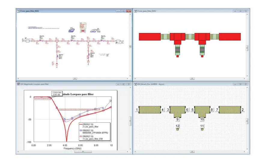
When using a circuit simulator without verification with an EM simulator, there are some physical aspects that are not taken into account. One should remember that the parametric-cell transmission line elements used in the circuit design (MLIN’s, MTEE’s etc) are mathematical models that assume ideal conditions without any coupling with surrounding elements. Obviously this is not the case in our example design and therefore we will have to perform a verification check on the copper layout to assure that there are no unforeseen side effects to our design. AWR Microwave Office facilitates two relatively easy ways of doing this. One can copy/paste the copper from the layout view to the simulator but a significantly easier and faster way is to run a script that will automatically configure the EM simulator based on the layout and substrate parameters. Next step is to ‘tell’ the software which elements should be included in the EM simulation and once this is done the EM simulated results will automatically replace the closed-form models and integrate the EM result into the existing schematic. For the remainder of this treatment we will use the simulations without the EM analysis as the results in Figure 4 are similar except for a better prediction of the finite minimum in transmission that is over predicted without EM analysis. The hashed red bars on the S21 graph in Figure 4 indicate yield specifications to be discussed in the next section.
Figure 3: Picture of Fabricated Design.
Yield Analysis
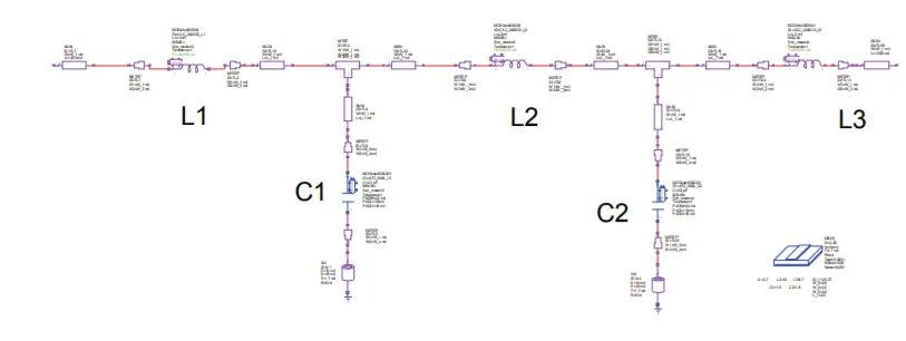
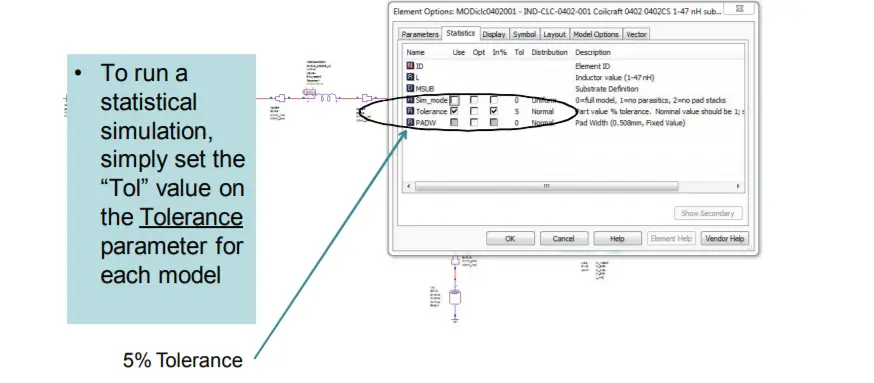
The design shown previously is now the starting point for our tolerance analysis. The focus will be on the tolerances of the surface mount L-C values. Figure 5 shows the filter design in the AWR design environment. To run statistics with Modelithics Global models, a tolerance parameter is enabled and assigned to the anticipated manufacturing distribution. Figure 6 shows one of the inductors selected and assigned to have a 5% normal or Gaussian distribution. In the first yield analysis, a 5% normal distribution will be assigned to the three inductors and the two capacitors used in the design.
Figure 4: Simulated Results for Nominal Filter achieved with and without the use of EM simulation, compared to measured results with looser tolerance parts (as compared to the measurements of Fig. 3). S11 (dB) – left, S21 (dB) – right. Blue lines ~ Measurements, Red lines ~ Modeled, Magenta ~ Modeled with EM Simulation of T-Line effects.
Figure 6: Example of assigning a tolerance parameter to an inductor
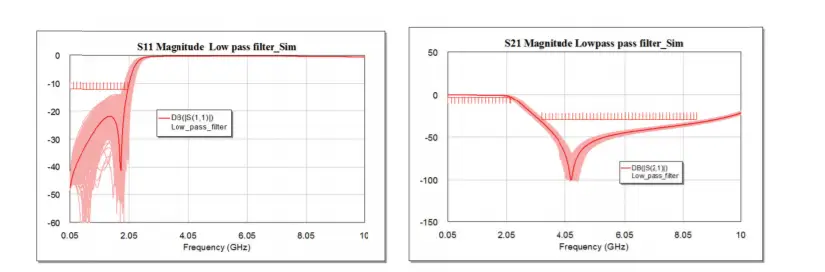
A yield analysis is then performed, using 500 iterations, which resulted with an initial yield of 54% for the design specifications shown earlier in table 1. These yield goals are setup as the limit bars on the graphs shown in Figure 7. The S11 and S21 results are also shown, with the nominal design being the dark line.
Figure 7: Initial yield analysis results – S11 (dB) left, S21 (dB) right. Dark line ~ nominal design. (Design specifications indicated by yield bars: |S11dB| < -12 from DC to 2.0 GHz, |S21dB| > -3 from DC to 2.2 GHz, |S21dB| < -30 from 3.25-8.5 GHz )
It is common practice for some components to have tight tolerance parts selected or “binned” from the middle of a manufacturing lot. This results in a bi-nominal or “normal with a gap” distribution if loose tolerance parts are purchased. This type of distribution can be simulated in AWR with a distribution called “Normal-Tol” which allows for specifying 2 values, one being the tight tolerance percentage that has been chopped out and the other being the overall manufacturing distribution the tight tolerance parts have been selected from. Using this type of distribution for all the L-C components actually reduces the yield to 45%. With this distribution, none of the design simulations will have nominal part values.
The tight tolerance parts that would have been selected from the middle of such a binned distribution approach would not really be Normal or Gaussian. To account for this, AWR has an inverse distribution called “Normal-Clipped”. If it is assumed that first only the capacitors, then only the inductors have this type of 2% tight tolerance (Normal-Clipped) distribution we can achieve slightly higher yields of 50% and 47%, respectively. If it is assumed that all the inductors and capacitors have this tight tolerance distribution, the yield can be increased to 85%; however this is an expensive design now. It would be prudent to find another way to reduce the cost and achieve this yield.
Sensitivity Analysis
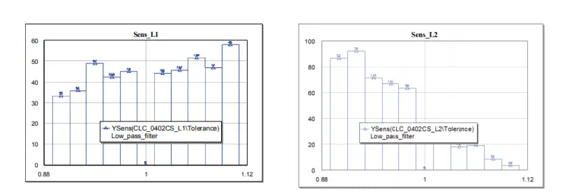
As a byproduct of yield analysis, the Microwave Office simulation can be setup to output sensitivity graphs for all the varied parameters. These graphs can help the user quickly identify which parameters the design performance is sensitive to and which it is not. It can also suggest a direction to change a parameter for improved yield and realize what is often referred to as “design centering”.
Figure 8: Sensitivity graphs for L1 (left) and L2 (right)
Figure 8 shows sensitivity graphs of the L1 and L2 inductors. The results shown are after 1000 iterations with 5/2% Normal-tol distributions for all components. In AWR Microwave Office the Yield Analysis output measurement parameter “YSens” is used to generate this information after setting up a rectangular graph. In using this output parameter with Modelithics Global models, it is recommended to set Ysens to the Tolerance parameter of the component of interest (and not the part value itself). From the data shown in Figure 8, we can see that the yield can be improved with a lower value of L2, while it seems less sensitive to L1. The analysis shows that the yield is reasonably centered on the “L1” value, but may provide better yield with a lower value of L2. Examination of the sensitivity graphs for the remaining parameters, not shown for brevity show that the design was reasonably centered or insensitive to the other component values.
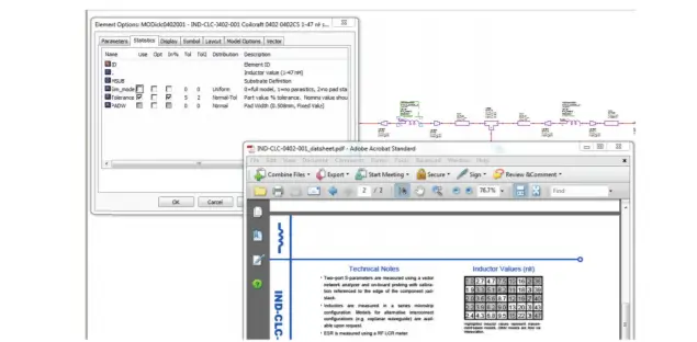
Understanding the results of the sensitivity analysis, it is possible explore how the yield results might change by lowering the value of L2 from its nominal value of 5.1nH. The Modelithics model datasheet is one way to identify the available discrete values the user might select as a substitution. On page 2 of the L2 inductor data sheet (shown in Figure 9), the next lower values from nominal (5.1nH) in the table are 4.7 and 4.3nH. The value 4.7nH was selected and the tolerance analysis repeated.
Figure 9: Accessing the model’s datasheet from the element options tab.
Yield Results After Sensitivity Analysis
The inductor value substitution resulted in immediate yield improvement. After changing L2 to 4.7nH, yield for the case of all 5% loose tolerance part values improved to 69% (up from 54%).
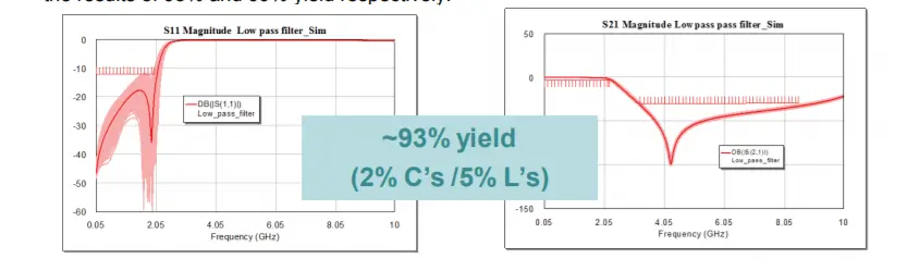
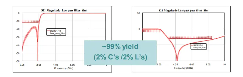
Further improvements to 80% and 93% are realized by using tighter 2% tolerance parts for inductors-only and capacitors-only, respectively. The use of tight tolerance parts for all inductors and capacitors produces a simulated yield of 100%, or 99% if we factor in 5% tolerances on the substrate height and dielectric constant and +/- 1 mil on line widths. Figures 10 and 11 show the results of 93% and 99% yield respectively.
Figure 10: S11 (left) and S21 (right) for a design with 93% yield.
Figure 11: S11 (left) and S21 (right) for a design with 99% yield.
Conclusion
This paper has illustrated a complete design flow along with the use of statistically enabled models yield and sensitivity analyses. It was shown that, starting with an ideal design, a nominal design that has good agreement to measurements can be achieved and then adjusted for improved yield accounting for anticipated manufacturing tolerances. This same design flow is NOT possible with S-Parameter models. Note 99% yield was achieve in principle, however, it should be noted that parameters varied did not include other assembly variations, such as parts placement and via uniformity. With looser 5% tolerance parts assumed there still was a yield improvement from 45% to 69% after design centering, and after adding 2% tolerance parts for the capacitors only yield improved from 50% to 93%.
About this note
This application note was developed by Larry Dunleavy and Lars van der Klooster (of Agetto MTT), with formatting and editing assistance by Laura Levesque and USF student intern, Scott Muir.
Contact Information
For information about Modelithics’ products and services, please contact Modelithics, Inc., 3650 Spectrum Blvd., Suite 170, Tampa, FL 33612 / Voice ~ 888-359-6539 / Email ~ sales@modelithics.com / Web ~ www.modelithics.com
References
[1] “Comprehensive Models for RLC Components to Accelerate PCB Designs,” Microwave Journal, May 2004.
[2] G. Matthaei, L. Young and E.M.T. Jones, Microwave Filters, Impedance-Matching Networks and Coupling Structures, 1964 McGraw Hill.
[3] AWR Corporation, 1960 E. Grand Avenue, Suite 430, El Segundo, CA 90245. http://web.awrcorp.com/